"Growing Artificial Societies" (Epstein & Axtell 1996) is a reference book for scientists interested in agent-based modelling and computer simulation. It represents one of the most paradigmatic and fascinating examples of the so-called generative approach to social science (Epstein 1999). In their book, Epstein & Axtell (1996) present a computational model where a heterogeneous population of autonomous agents compete for renewable resources that are unequally distributed over a 2-dimensional environment. Agents in the model are autonomous in that they are not governed by any central authority and they are heterogeneous in that they differ in their genetic attributes and their initial environmental endowments (e.g. their initial location and wealth). The model grows in complexity through the different chapters of the book as the agents are given the ability to engage in new activities such as sex, cultural exchange, trade, combat, disease transmission, etc. The core of Sugarscape has provided the basis for various extensions to study e.g. norm formation through cultural diffusion (Flentge et al. 2001) and the emergence of communication and cooperation in artificial societies (Buzing et al. 2005). Here we analyse the model described in the second chapter of Epstein & Axtell's (1996) book within the Markov chain framework.
The first model that Epstein & Axtell (1996) present comprises a finite population of agents who live in an environment. The environment is represented by a two-dimensional grid which contains sugar in some of its cells, hence the name Sugarscape. Agents' role in this first model consists in wandering around the Sugarscape harvesting the greatest amount of sugar they can find.
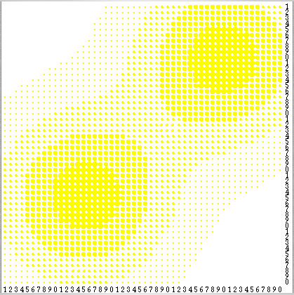
The environment is a 50×50 grid that wraps around forming a torus. Grid cells have both a sugar level and a sugar capacity c. A cell's sugar level is the number of units of sugar in the cell (potentially none), and its sugar capacity c is the maximum value the sugar level can take on that cell. Sugar capacity is fixed for each individual cell and may be different for different cells. The spatial distribution of sugar capacities depicts a sugar topography consisting of two peaks (with sugar capacity c = 4) separated by a valley, and surrounded by a desert region of sugarless cells (see Figure 1) –note, however, that the grid wraps around in both directions–.
| Figure 1. Spatial distribution of sugar capacities in the Sugarscape. Cells are coloured according to their sugar capacity c: cells with c = 0 are white, whereas cells with c > 0 contain a yellow circle whose radius is proportional to the cell's capacity c. Sugar capacity ranges from 0 to 4. Source: Epstein & Axtell (1996). |
The Sugarscape obbeys the following rule:
Every agent is endowed with individual (life-long) characteristics that condition her skills and capacities to survive in the Sugarscape. These individual attributes are:
Agents also have the capacity to accumulate sugar wealth w. An agent's sugar wealth is incremented at the end of each time-step by the sugar collected and decremented by the agent's metabolic rate. Two agents are not allowed to occupy the same cell in the grid.
The agents' behaviour is determined by the following two rules:
Scheduling is determined by the order in which the different rules G, M and R are fired in the model. Environmental rule G comes first, followed by agent rule M (which is executed by all agents in random order) and finally agent rule R is executed (again, by all agents in random order).
Our analysis corresponds to a model used by Epstein & Axtell (1996, pg. 33) to study the emergent wealth distribution in the agent population. This model is parameterised as indicated in Table 1 below (where U[a,b] denotes a uniform distribution with range [a,b]).
| Lattice length L | 50 |
| Cells' sugar capacity distribution | See Figure 1 |
| Growth rate α | 1 |
| Number of agents N | 250 |
| Agents' initial wealth w0 distribution | U[5,25] |
| Agents' metabolic rate m distribution | U[1,4] |
| Agents' vision v distribution | U[1,6] |
| Agents' maximum age max-age distribution | U[60,100] |
| Table 1. Model parameterisation. |
Initially, each cell of the Sugarscape contains a sugar level equal to its sugar capacity c, and the 250 agents are created at a random unoccupied initial location and with random attributes (using the uniform distributions indicated in Table 1 above).
Sugarscape parameterised as indicated above can be represented as a time-homogeneous Markov chain (THMC) defining the state of the system as a 50×50 array where each element corresponds to one cell of the grid and stores the following information: the cell's sugar level and, if the cell is occupied, the agent's vision, metabolic rate, wealth and life expectancy (i.e. the agent's maximum age minus the agent's current age). With this definition, the number of possible states is the number of possible combinations of these variables that can be reached by running the model. Note that the state space is finite since all the state variables can only take a finite set of values.
The system so defined is a THMC because given any particular state the probability distribution over the state space for the following time-step is fully determined. The state space is quite large, but this neither impedes nor limits our analysis; as usual, the important point is not to fully characterise the transition matrix but to adequately partition the state space as indicated in Proposition 2.
Here we argue that the state space of the induced THMC described in the previous section is irreducible and aperiodic (also called ergodic). The demonstration of this statement relies on the existence of what we call regenerating states. These are states where agents stay stationary and no sugar is collected. Any state where every agent has vision v = 1 and all (250) agents are placed in any of the 305 locations colured in red in figure 2 is regenerating. These red locations are the cells with sugar capacity c = 0 and whose neighbouring cells' sugar capacity c is also 0. Agents do not move because the only unoccupied cells they can see have no sugar, and no sugar is collected for the same reason. Any regenerating state can be succeeded by another regenerating state. To achieve that, one only has to place any newborn in one of the 305 locations coloured in red in figure 2. Thus, by moving from one regenerating state to another we can bring the environment back to a pristine state where every cell's sugar level is equal to its capacity, hence the adjective regenerating.
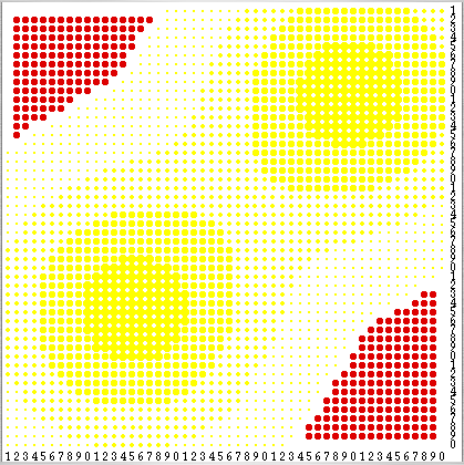
| Figure 2. Any state where every agent's vision v is equal to 1 and all (250) agents are placed in any of the 305 locations colured in red is regenerating. |
Some regenerating states are particularly important for our analysis. These are called exterminating pristine states because they fulfil two additional conditions:
Having explained what exterminating pristine states are, we prove that the THMC is irreducible, i.e. it is possible to go from any state i to any state j in a finite number of time-steps. The proof [1] rests on the following facts:
Having proved that the THMC is irreducible, it only remains to prove that it is also aperiodic. To prove this it suffices to find an aperiodic state –as indicated in section 8 of our paper, after definition 7–. Note that any exterminating pristine state ext-prist-st is clearly aperiodic, since the greatest common divisor of the set of integers n such that p(n)ext-prist-st,ext-prist-st > 0 is 1, as explained in the third bullet point of the previous list.
This concludes the proof that the induced THMC is irreducible and aperiodic, i.e. ergodic. As we have seen in the paper, in ergodic THMCs the probability of finding the system in each of its states in the long run is strictly positive and independent of the initial conditions, and the limiting distribution π coincides with the occupancy distribution π* (the long-run fraction of time that the system spends in each state). Hence, the limiting distribution of any statistic (e.g. the sugar wealth distribution) coincides with its occupancy distribution too, and does not depend on the initial conditions. Thus, we could approximate the limiting distribution of emergent wealth distributions in Sugarscape as much as we like by running just one simulation (with any initial conditions) for long enough.
BUZING P, Eiben A & Schut M (2005) Emerging communication and cooperation in evolving agent societies. Journal of Artificial Societies and Social Simulation 8(1)2. https://www.jasss.org/8/1/2.html.
EPSTEIN J M (1999) Agent-Based Computational Models And Generative Social Science. Complexity 4(5), pp. 41-60.
EPSTEIN J M & Axtell R L (1996) Growing Artificial Societies: Social Science from the Bottom Up. The MIT Press.
FLENTGE F, Polani D & Uthmann T (2001) Modelling the emergence of possession norms using memes. Journal of Artificial Societies and Social Simulation 4(4)3. https://www.jasss.org/4/4/3.html.
1 The procedure used here to prove that something is possible consists in identifying a sequence of random events that can occur with strictly positive probability.